
Quite often, as Database Administrators we are faced the case, when our attitude to SQLs, our knowledge of topic, is in contraty to what Developers know..
It all comes from fact, that Developers, do not have some information, and look at application from functional point of view…
In this series of posts, I will try to build a bridge between DBAs and DEVs…
So, let’s go to the point..
Subjects that this series will raise:
- Selectivity / Cardinality and Histograms
- How to read execution plans (Explain Plan – sometimes lies ?)
- What is Shared pool – why Devs should know it ?
- Bind variables vs Literals
- Variable Bind Peeking
- Adaptive Cursor Sharing – selectivity cubes
- Access Paths and Join Methods
- Result Set Cache
- Adaptive Optimizations in 12c
Selectivity
Two main terms are Selectivity and Cardinality
- Row Source – can be a table, can be a result of join operation, in general is a result of execution plan step
- Selectivity represents a fraction of rows from a row source
- What influences Selectivity
- I/O cost
- Sort cost
- Lies in a value range from 0.0 through 1.0
How Selectivity is estimated ?
Each object in database should have statistics about data. This statistics are a base for Oracle Cost Optimizer to estimate Selectivity of Row Source. When statistics are not available, the estimator uses default values or dynamic sampling.
Examples of statistics data are:
- Number of Rows
- Average Row Length
- Number of distinct values
Skewed Data and Histograms
Example of skewed data is a column that contains 3 distinct values. Value 1 and 2 is evenly distriuted and value num 3 is very rare…
With this kind of data, knowing only the number of distinct values, cannot lead to accurate assumption of data selectivity of value 3.
And here comes the Histograms
Height-Balanced Histograms – uniform Distribution
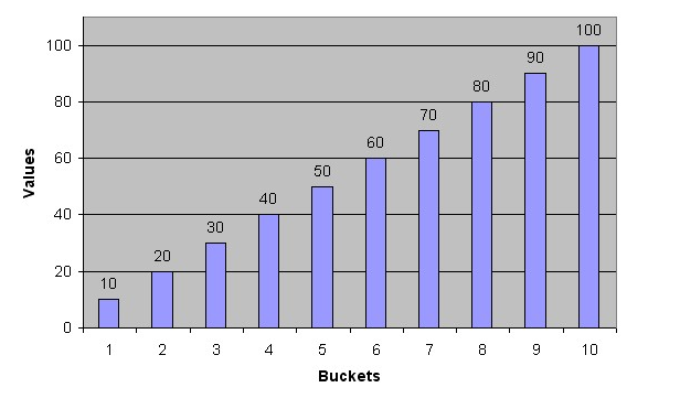
Consider a column C with values between 1 and 100 and a histogram with 10 buckets.
If the data in C is uniformly distributed, then the histogram looks similar to this one, where the numbers are the endpoint values.
The number of rows in each bucket is one tenth the total number of rows in the table.
Four-tenths of the rows have values that are between 60 and 100 in this example of uniform distribution.
Height-Balanced Histograms – Non-uniform Distribution
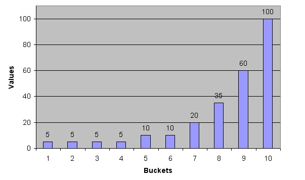
In this case, most of the rows have the value 5 for the column. Only 1/10 of the rows have values between 60 and 100.
Frequency Histograms
In a frequency histogram, each value of the column corresponds to a single bucket of the histogram.
Each bucket contains the number of occurrences of that single value.
Why histograms are so important ,and Devs should care about them ?
- They are the only way to deal with skewed data
- Are prerequisite for mechanism called Bind Variable Peeking (introduced in Oracle 9i)
We will talk about it , and play with it in next part of this series
Reading Execution Plans – quick review
Not to bore you only with theory, now it is time to quick review of reading execution plans
First let’s create test table, with simple skewed data
create user tstuser identified by tstuser default tablespace USERS;
grant dba to tstuser;
connect tstuser/tstuser
create table tab1_plan as select level "ID", 'descr:' || level "DESCR" from dual connect by level <= 1000000;
alter table tab1_plan add sex char(3);
update tab1_plan set sex='M' where id between 1 and 700000;
update tab1_plan set sex='F' where id between 700001 and 999000;
update tab1_plan set sex='N' where id between 999001 and 1000000;
update tab1_plan set sex='N/A' where id=1000000;
create index TAB1_PLAN_SEX on TAB1_PLAN(SEX);
First we create test user, and give him dba role, just because I’m a lazy bastard..:)
Then create table tab1_plan, with column id, description. Then we add column “sex” with four distinct values od sex M – male, F – female, N – Neutral, N/A – Not Available data.
Next create an index tab1_plan_sex on skewed data column.
Let’s gather statistics with histograms on skewed data
exec dbms_stats.gather_table_stats(ownname=>'TSTUSER',tabname=>'TAB1_PLAN',method_opt=>'FOR ALL INDEXED COLUMNS',estimate_percent=>100,cascade=>true);
col TABLE_NAME format a40
col COLUMN_NAME format a40
set lines 200
select TABLE_NAME,COLUMN_NAME,HISTOGRAM from dba_tab_col_statistics where table_name = 'TAB1_PLAN';

TABLE_NAME                               COLUMN_NAME                              HISTOGRAM
---------------------------------------- ---------------------------------------- ---------------
TAB1_PLAN                                SEX                                      FREQUENCY
TAB1_PLAN                                DESCR                                    NONE
TAB1_PLAN                                ID                                       NONE
We already have test table.
Lets define bind variable, to compare different ways to see execution plan.
var b_sex char(3);
exec :b_sex := 'M'
explain plan for select avg(id) from tab1_plan where sex=:b_sex;
The most basic way to see execution plan is to use Explain Plan feature.
But remember, Explain Plan, only does parsing ..! It means , as you will see later it can show incorrect execution plan.
Explain plan stores results in special table called PLAN_TABLE. To see the results from PLAN_TABLE you can use
dbms_xplan.display function
select * from table(dbms_xplan.display);
PLAN_TABLE_OUTPUT
--------------------------------------------------------------------------------
Plan hash value: 2103054430

--------------------------------------------------------------------------------
| Id  | Operation          | Name      | Rows  | Bytes | Cost (%CPU)| Time     |
--------------------------------------------------------------------------------
|   0 | SELECT STATEMENT   |           |     1 |     9 |  1081   (1)| 00:00:01 |
|   1 |  SORT AGGREGATE    |           |     1 |     9 |            |          |
|*  2 |   TABLE ACCESS FULL| TAB1_PLAN |   250K|  2197K|  1081   (1)| 00:00:01 |

Predicate Information (identified by operation id):
---------------------------------------------------

2 - filter("SEX"='M')
Assigning value to b_sex variable we have chosen very non-selective value “M”. As we could expect access path is full scan.
Lets change the value to very selective value
exec :b_sex := 'N/A'
explain plan for select avg(id) from tab1_plan where sex=:b_sex;
select * from table(dbms_xplan.display);

PLAN_TABLE_OUTPUT
--------------------------------------------------------------------------------------------------------------------------------------------------------------------------------------------------------
Plan hash value: 2103054430

--------------------------------------------------------------------------------
| Id  | Operation          | Name      | Rows  | Bytes | Cost (%CPU)| Time     |
--------------------------------------------------------------------------------
|   0 | SELECT STATEMENT   |           |     1 |     9 |  1081   (1)| 00:00:01 |
|   1 |  SORT AGGREGATE    |           |     1 |     9 |            |          |
|*  2 |   TABLE ACCESS FULL| TAB1_PLAN |   250K|  2197K|  1081   (1)| 00:00:01 |
Explain plan is still showing full table scan..
So, let’s run the query
select avg(id) from tab1_plan where sex=:b_sex;
select * from table(dbms_xplan.display_cursor(format=>'allstats last +PEEKED_BINDS'));

SQL_ID 1pfqnxjdm8spq, child number 0
-------------------------------------
select avg(id) from tab1_plan where sex=:b_sex

Plan hash value: 2424300629

-----------------------------------------------------------------------
| Id  | Operation                            | Name          | E-Rows |
-----------------------------------------------------------------------
|   0 | SELECT STATEMENT                     |               |        |
|   1 |  SORT AGGREGATE                      |               |      1 |
|   2 |   TABLE ACCESS BY INDEX ROWID BATCHED| TAB1_PLAN     |      1 |
|*  3 |    INDEX RANGE SCAN                  | TAB1_PLAN_SEX |      1 |
-----------------------------------------------------------------------

Peeked Binds (identified by position):
--------------------------------------

   1 - :1 (CHAR(30), CSID=873): 'N/A'
So what’s happened ? We will come back to it when we will be talking about bind peeking…
For now, you should remember:
- EXPLAIN PLAN does only parsing
- You can see real execution plan from Cursor with dbms_xplan package display_cursor function
What is this Cursor from the connected session point of view ?? Still must be patient …:) we will come back to it 🙂
DBMS_XPLAN Package
The DBMS_XPLAN package supplies five table functions.
For Devs most important are:
DISPLAY – to format and display the contents of a plan table.
DISPLAY_CURSOR – to format and display the contents of the execution plan of any loaded cursor
You have already seen how to get execution plan from PLAN_TABLE with dbms_xplan.display function .
Let’s concentrate on displaying execution plan for specific Cursor
First let’s generate few execution plans for our query
SET PAGESIZE 0
SET LINES 300

exec :b_sex:='M'
select /* DISP_LAST */ avg(id) from tab1_plan where sex=:b_sex;
select /* DISP_LAST */ avg(id) from tab1_plan where sex=:b_sex;

exec :b_sex:='N/A'
select /* DISP_LAST */ avg(id) from tab1_plan where sex=:b_sex;
select /* DISP_LAST */ avg(id) from tab1_plan where sex=:b_sex;
select /* DISP_LAST */ avg(id) from tab1_plan where sex=:b_sex;
select /* DISP_LAST */ avg(id) from tab1_plan where sex=:b_sex;

exec :b_sex:='N'
select /* DISP_LAST */ avg(id) from tab1_plan where sex=:b_sex;
select /* DISP_LAST */ avg(id) from tab1_plan where sex=:b_sex;
select /* DISP_LAST */ avg(id) from tab1_plan where sex=:b_sex;
select /* DISP_LAST */ avg(id) from tab1_plan where sex=:b_sex;
To display execution plan for last run of query in current session
 select * from table(dbms_xplan.display_cursor());

SQL_ID 0a9wfq8qtn4qf, child number 0
-------------------------------------
select /* DISP_LAST */ avg(id) from tab1_plan where sex=:b_sex
Plan hash value: 2103054430

--------------------------------------------------------------------------------
| Id  | Operation          | Name      | Rows  | Bytes | Cost (%CPU)| Time     |
--------------------------------------------------------------------------------
|   0 | SELECT STATEMENT   |           |       |       |  1086 (100)|          |
|   1 |  SORT AGGREGATE    |           |     1 |     9 |            |          |
|*  2 |   TABLE ACCESS FULL| TAB1_PLAN |   700K|  6152K|  1086   (2)| 00:00:01 |
--------------------------------------------------------------------------------

Predicate Information (identified by operation id):
---------------------------------------------------

   2 - filter("SEX"=:B_SEX)
Let’s display what other plans are generated for our query . We can you ie. SQL ID returned from last run of display_cursor, and v$sql view
which keeps all parsed Cursors from shared pool (library cache)
Select SQL_ID,CHILD_NUMBER,PLAN_HASH_VALUE,SUBSTR(SQL_TEXT,1,40) from v$sql where SQL_ID='0a9wfq8qtn4qf';
0a9wfq8qtn4qf 0 2103054430 select /* DISP_LAST */ avg(id) from tab
0a9wfq8qtn4qf 1 2424300629 select /* DISP_LAST */ avg(id) from tab
0a9wfq8qtn4qf 2 2424300629 select /* DISP_LAST */ avg(id) from tab
So, we have two different plans (2103054430, 2424300629), and three Child Cursors.
Display execution plan for child number 1
select * from table(dbms_xplan.display_cursor(sql_id=>'0a9wfq8qtn4qf',cursor_child_no=>1,format=>'BASIC'));
EXPLAINED SQL STATEMENT:

select /* DISP_LAST */ avg(id) from  tab1_plan where sex=:b_sex

Plan hash value: 2424300629

--------------------------------------------------------------
| Id  | Operation                            | Name          |
--------------------------------------------------------------
|   0 | SELECT STATEMENT                     |               |
|   1 |  SORT AGGREGATE                      |               |
|   2 |   TABLE ACCESS BY INDEX ROWID BATCHED| TAB1_PLAN     |
|   3 |    INDEX RANGE SCAN                  | TAB1_PLAN_SEX |
--------------------------------------------------------------
As you already could notice, there is a parameter “format”
By default its value is “TYPICAL” . Displays the most relevant information in the plan (operation id, name and option, #rows, #bytes and optimizer cost).
Pruning, parallel and predicate information are only displayed when applicable. Excludes only PROJECTION, ALIAS and REMOTE SQL information
SQL> select * from table(dbms_xplan.display_cursor(sql_id=>'0a9wfq8qtn4qf',cursor_child_no=>1,format=>'TYPICAL'));
SQL_ID 0a9wfq8qtn4qf, child number 1
-------------------------------------
select /* DISP_LAST */ avg(id) from  tab1_plan where sex=:b_sex

Plan hash value: 2424300629

------------------------------------------------------------------------------------------------------
| Id  | Operation                            | Name          | Rows  | Bytes | Cost (%CPU)| Time     |
------------------------------------------------------------------------------------------------------
|   0 | SELECT STATEMENT                     |               |       |       |     4 (100)|          |
|   1 |  SORT AGGREGATE                      |               |     1 |     9 |            |          |
|   2 |   TABLE ACCESS BY INDEX ROWID BATCHED| TAB1_PLAN     |     1 |     9 |     4   (0)| 00:00:01 |
|*  3 |    INDEX RANGE SCAN                  | TAB1_PLAN_SEX |     1 |       |     3   (0)| 00:00:01 |
------------------------------------------------------------------------------------------------------

Predicate Information (identified by operation id):
---------------------------------------------------

   3 - access("SEX"=:B_SEX)
“Format” value of “ALL” is maximum level. Includes information displayed with the TYPICAL level with additional information (PROJECTION, ALIAS and information about REMOTE SQL if the operation is distributed).
Not all information are relevant, for example PROJECTION is Exadata specific.It displays sth called query blocks , and they are beyond of this topic.
 SQL> select * from table(dbms_xplan.display_cursor(sql_id=>'0a9wfq8qtn4qf',cursor_child_no=>1,format=>'ALL'));
SQL_ID 0a9wfq8qtn4qf, child number 1
-------------------------------------
select /* DISP_LAST */ avg(id) from  tab1_plan where sex=:b_sex

Plan hash value: 2424300629

------------------------------------------------------------------------------------------------------
| Id  | Operation                            | Name          | Rows  | Bytes | Cost (%CPU)| Time     |
------------------------------------------------------------------------------------------------------
|   0 | SELECT STATEMENT                     |               |       |       |     4 (100)|          |
|   1 |  SORT AGGREGATE                      |               |     1 |     9 |            |          |
|   2 |   TABLE ACCESS BY INDEX ROWID BATCHED| TAB1_PLAN     |     1 |     9 |     4   (0)| 00:00:01 |
|*  3 |    INDEX RANGE SCAN                  | TAB1_PLAN_SEX |     1 |       |     3   (0)| 00:00:01 |
------------------------------------------------------------------------------------------------------

Query Block Name / Object Alias (identified by operation id):
-------------------------------------------------------------

   1 - SEL$1
   2 - SEL$1 / TAB1_PLAN@SEL$1
   3 - SEL$1 / TAB1_PLAN@SEL$1

Predicate Information (identified by operation id):
---------------------------------------------------

   3 - access("SEX"=:B_SEX)

Column Projection Information (identified by operation id):
-----------------------------------------------------------

   1 - (#keys=0) AVG("ID")[22]
   2 - "ID"[NUMBER,22]
   3 - "TAB1_PLAN".ROWID[ROWID,10]
Looking at these execution plans, still we do not know what value of bind variable was selected..
“Format” parameter has lot of “extensions”, some of them are undocumented…
Display bind values
select * from table(dbms_xplan.display_cursor(sql_id=>'0a9wfq8qtn4qf',cursor_child_no=>1,format=>'TYPICAL +PEEKED_BINDS'));

SQL_ID 0a9wfq8qtn4qf, child number 1
-------------------------------------
select /* DISP_LAST */ avg(id) from  tab1_plan where sex=:b_sex

Plan hash value: 2424300629

------------------------------------------------------------------------------------------------------
| Id  | Operation                            | Name          | Rows  | Bytes | Cost (%CPU)| Time     |
------------------------------------------------------------------------------------------------------
|   0 | SELECT STATEMENT                     |               |       |       |     4 (100)|          |
|   1 |  SORT AGGREGATE                      |               |     1 |     9 |            |          |
|   2 |   TABLE ACCESS BY INDEX ROWID BATCHED| TAB1_PLAN     |     1 |     9 |     4   (0)| 00:00:01 |
|*  3 |    INDEX RANGE SCAN                  | TAB1_PLAN_SEX |     1 |       |     3   (0)| 00:00:01 |
------------------------------------------------------------------------------------------------------

Peeked Binds (identified by position):
--------------------------------------

   1 - :B_SEX (CHAR(30), CSID=873): 'N/A'

Predicate Information (identified by operation id):
---------------------------------------------------

   3 - access("SEX"=:B_SEX)
Now, you see, that bind value for this executios of Cursor was ‘N/A’
Very interesting feature is displaying IO statistics … Not rare statistics can lead optimizer to wrong assumptions about cardinality ..
It is sometimes worth to check reality versus optimizer assumptions
To check it, we will use GATHER_PLAN_STATISTICS hint and “ALLSTATS” extention of format parameter.
exec :b_sex:='N/A'
select /* DISP_IOSTATS */ /*+ GATHER_PLAN_STATISTICS */ avg(id) from tab1_plan where sex=:b_sex;
select * from table(dbms_xplan.display_cursor(format=>'ALL LAST +ALLSTATS +PEEKED_BINDS'));
SQL_ID 8470tyjk6ftub, child number 1
-------------------------------------
select /* DISP_IOSTATS */ /*+ GATHER_PLAN_STATISTICS */ avg(id) from
tab1_plan where sex=:b_sex

Plan hash value: 2424300629

--------------------------------------------------------------------------------------------------------------------------
| Id  | Operation          | Name      | Starts | E-Rows |E-Bytes| Cost (%CPU)| E-Time   | A-Rows |   A-Time   | Buffers |
--------------------------------------------------------------------------------------------------------------------------
|   0 | SELECT STATEMENT   |           |      1 |        |       |  1086 (100)|          |      1 |00:00:00.04 |    3905 |
|   1 |  SORT AGGREGATE    |           |      1 |      1 |     9 |            |          |      1 |00:00:00.04 |    3905 |
|*  2 |   TABLE ACCESS FULL| TAB1_PLAN |      1 |    700K|  6152K|  1086   (2)| 00:00:01 |      1 |00:00:00.04 |    3905 |
--------------------------------------------------------------------------------------------------------------------------


Query Block Name / Object Alias (identified by operation id):
-------------------------------------------------------------

   1 - SEL$1
   2 - SEL$1 / TAB1_PLAN@SEL$1

Peeked Binds (identified by position):
--------------------------------------

   1 - :1 (CHAR(30), CSID=873): 'M  '

Predicate Information (identified by operation id):
---------------------------------------------------

   2 - filter("SEX"=:B_SEX)

Column Projection Information (identified by operation id):
-----------------------------------------------------------

   1 - (#keys=0) AVG("ID")[22]
   2 - "ID"[NUMBER,22]
Now we see two pairs of additional columns “E-Rows”, “A-Rows”, and “E-Time” , “A-Time”..
“A” stands for Actuall, and “E” stands for Estimated…
So in step 2 optimizer assumed to get 700K rows, that’s why has choosen FULL SCAN instead of index access, and A-Rows was “1”
Last way of looking at execution plans , but firstly on Execution Statistics is AUTOTRACE feature.
set lines 300
set pages 0
set autotrace traceonly
select avg(id) from tab1_plan where sex='N';

Execution Plan
----------------------------------------------------------
Plan hash value: 2424300629

------------------------------------------------------------------------------------------------------
| Id  | Operation                            | Name          | Rows  | Bytes | Cost (%CPU)| Time     |
------------------------------------------------------------------------------------------------------
|   0 | SELECT STATEMENT                     |               |     1 |     9 |     9   (0)| 00:00:01 |
|   1 |  SORT AGGREGATE                      |               |     1 |     9 |            |          |
|   2 |   TABLE ACCESS BY INDEX ROWID BATCHED| TAB1_PLAN     |   999 |  8991 |     9   (0)| 00:00:01 |
|*  3 |    INDEX RANGE SCAN                  | TAB1_PLAN_SEX |   999 |       |     5   (0)| 00:00:01 |
------------------------------------------------------------------------------------------------------

Predicate Information (identified by operation id):
---------------------------------------------------

   3 - access("SEX"='N')


Statistics
----------------------------------------------------------
          1  recursive calls
          0  db block gets
        172  consistent gets
          0  physical reads
          0  redo size
        542  bytes sent via SQL*Net to client
        551  bytes received via SQL*Net from client
          2  SQL*Net roundtrips to/from client
          0  sorts (memory)
          0  sorts (disk)
          1  rows processed
“set autotrace traceonly” parses our query , executes it, prevents output and displays executions statistics.
Execution plan is the same as form Explain Plan. but statistics are real one .
other example of using Autotrace is displaying only statistics
set autotrace traceonly statistics
select avg(id) from tab1_plan where sex='N';

Statistics
----------------------------------------------------------
1 recursive calls
0 db block gets
172 consistent gets
0 physical reads
0 redo size
542 bytes sent via SQL*Net to client
551 bytes received via SQL*Net from client
2 SQL*Net roundtrips to/from client
0 sorts (memory)
0 sorts (disk)
1 rows processed
The same information you can get eg. V$SQL view
It is time to talk about these mysterious Cursors, Shared Pool , Parsing , Adaptive Optimizations …but in part 2 of this series 🙂